Articles in this series:
Linearity (this page)
In the previous post I looked at dark frames. I will now look at the linearity of the QHY183M.
With my previous camera I did not actually do a linearity test, because I did not have a way of providing a constant light source. But this time I took Arne’s advice in his QHY600 posts to use a pulsed LED.
The illumination for these tests were from an LED run by an Arduino Uno. I wrote a little blinker program to pulse the LED a specified number of times. Each pulse is 1ms ON followed by 10ms OFF to avoid the LED heating up and changing brightness. More information about the test circuit and blinker program is here.
The median ADU of a 100×100 pixel region at the centre of the sensor is then plotted against the number of pulses. Here’s the result:
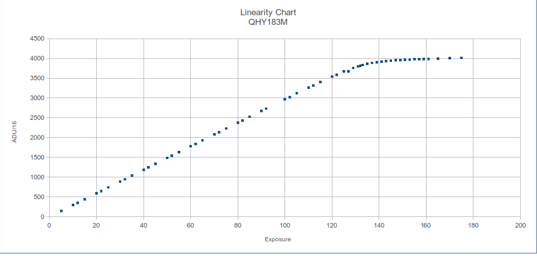
Somewhere above 3500 ADU there is a rollover as saturation kicks in. I now want to focus on the linear region to assess how good the linearity is, and to find the max ADU that is still in the linear region.


The linearity of the sensor is very impressive. There is an excellent straight line fit all the way to about 3,500 ADU (remember these are 12-bit ADUs – the actual number the camera will output is 3,500 x 16 = 56,000).
The residuals (against the straight line) plot show more detail. The rightmost point is ADU = 3,403. It looks like there is already some rollover here and in the previous point, which is ADU = 3,318. This is where saturation starts, so I will be limiting observations to ADU = 3,300.
On the residuals chart, you will also see 2 groups of points. One above the x-axis, and the other mostly below. These actually reflect how I ran the test. I started at the leftmost point, and increased the pulse count all the way to saturation. These are the points above the axis. I then reduced the pulses, picking different pulse counts on the way down. These are the lower points. With a perfect system these should all lie on the same line, but they don’t. I can only speculate why that might be. The LED was held in a 2″ eyepiece barrel, and there was tracing paper at the bottom of that barrel to act as a diffuser. Perhaps the position of the LED changed, or the paper shifted. The QHY183M also has a sensor window anti-fog heater, so maybe it got warmer as the test progressed.
In any case the effect is small. At 3,000 ADU the residuals are +-3 ADU, or 1ppt. Another way of looking at it is that 3,000 ADU corresponds to 3000 x Gain = 3000 x 3.78 = 11,340 e-. The shot noise contribution from this is SQRT(11,340) = 106 e- = 28 ADU.
Overall I am very pleased with this sensor. Low noise (read noise = 2.7 e-, an order of magnitude better than my ST-8XME) and excellent linearity.